Raytracing

1. Illumination

• Direct Illumination: surface point recieves light directly from all light sources in the scene.
• Global Illumination: surface point recieves light after rays interact with other objects in the scene (also computes shadows, reflections, refractions, etc).

2. Raycasting

A basic raycasting algorithm would:

1. For each pixel, generate a ray from the camera through the pixel into the scene.
2. For each ray, check for intersections with objects in the scene.
3. If an intersection is found, compute the color of the pixel based on the material properties of the object and the lighting in the scene.
4. If no intersection is found, set the pixel color to the background color.
5. Repeat for all pixels.

3. Raytracing

A raytracer would also include additional features such as:

• Shadows: by casting shadow rays from the intersection point to the light sources to determine if the point is in shadow.
• Reflections: by casting reflection rays from the intersection point to compute the color contribution based on the material's reflectivity.
• Refractions: by casting refraction rays from the intersection point to compute the color contribution based on the material's index of refraction.

This is a recursive algorithm. We can stop at a maximum recursion depth, or if reflected or transmitted contribution is below a certain threshold.

For each ray, we test which objects intersect the ray. If the object intersects we calculate the distance between viewpoint and intersection. The smallest distance is the visible surface. At that point, local illumination is computed as before, .

3.1 Secondary Rays

Secondary rays originate at intersection points, caused by reflections, refractions and shadows: .

Floating point precision errors can cause artifacts such as shadow acne (self-shadowing) and light leaks (missed shadows). To mitigate this, we can use a small bias (in the correct direction)when generating secondary rays.

• The object has a reflection coefficient that determines how much light is reflected. The mirror reflection direction is symmetrical with respect to the normal: where is the incoming ray direction and is the unit surface normal.
• The object has a transparency coefficient that determines how much light is transmitted through the object. The refraction direction is computed using Snell's law: where and are the indices of refraction of the two media, and and are the angles of incidence and refraction, respectively. So, the direction of the refracted ray is:

3.2 Fresnel Factor

Instead of having and as constants, we can compute them based on the angle of incidence using the Fresnel equations, such that . Fresnel equations provide more reflection at grazing angles, and less reflection at normal incidence.

The Fresnel coefficient can be approximated using Schlick's approximation:

Where is the Fresnel coefficient at normal incidence, a property of the material .

3.3 Shadows

When hitting a surface point, we also create a shadow ray from the surface point to each light source. If any object intersects the shadow ray, then the point is in shadow and only receives ambient light. So, if this ray hit is :

For soft shadows, we need an area light source, to which we can cast multiple shadow rays to different points on the light source, and average the results to .

3.4 Glossy Objects

Real scenes have glossy objects, which have a blurred reflection. To model this, we can cast multiple reflection rays in a cone around the mirror reflection direction, and average the results.

3.5 Monte-Carlo Raytracing

In Monte Carlo Raytracing, we case a ray form the eye to each pixels, then randomly cast rays in the hemisphere above the surface point, and average the results to compute the color of the pixel. This can be used to simulate global illumination, including indirect lighting, caustics, etc. This is a very computationally expensive method, but it can produce very realistic results.

We could also do several primary rays per pixel to reduce noise, and only cast 1 secondary ray per intersection to reduce the computational cost. This is called path tracing. This is more efficient than Monte Carlo raytracing, and produces better results.

4. Intersection Calculations

For each ray we must calculate all possible intersections with each object in the viewing volume. A ray can be described parametrically with origin and direction as . The direction vector itself can be calculated from the viewpoint as .

• is the part of the ray behind the viewing plane. All intersection points must have to be visible.
• is the part of the ray in front of the viewing plane.

4.1 Ray-Sphere Intersection

A point on the surface of a sphere satisfies where is the center of the sphere and is the radius. Substituting gives a quadratic equation in : . Setting we get:

• If has no solutions, there is no intersecton.
• If has one solution, the ray is tangent to the sphere.
• If has two solutions, the ray intersects the sphere at two points. We take the smaller positive solution (the closer point) as the intersection point.

Make sure to use an epsilon tolerence check to avoid floating point precision issues when checking for solutions.

4.2 Ray-Cylinder Intersection

To calculate the intersection with a cylinder we can use where and are the endpoints of the cylinder, , and is a vector perpendicular to . is the parameter along the cylinder axis, and is the parameter along the ray. Since , we can say:

And by substitution, and then knowing that :

After solving for , we can find , as:

• If then intersection is on the outside surface of the cylinder.
• If then intersection is on the inside surface of the cylinder.

4.3 Ray-Plane Intersection

The intersection of a ray with a plane is given by where is a point on the plane, is a vector on the plane. Given a plane normal , and knowing , we can solve for as:

4.4 Ray-Triangle Intersection

To calculate intersections, we want to test whether the triangle is front facing, whether its plane intersects the ray, and whether the intersection point is inside the triangle.

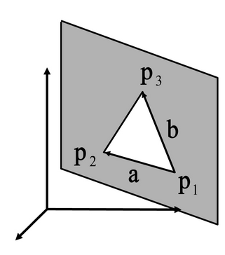
1. The triangle is front facing if where is the triangle normal. If then the ray is parallel to the triangle plane, and there is no intersection.
2. To calculate the plane equation, use and to get . Then perform ray-plane intersection as above to get intersection point .
3. To check if is inside the triangle, we can express where and are the triangle edges. Then, we check if , , and . We can calculate and using:

4.4.1 Moller Trumbore Algorithm

Instead of computing the plane equation, we can do:

1bool triangle_interection(vec3 v1, vec3 v2, vec3 v3, vec3 origin, vec3 dir, float* out) {
2  vec3 edge1 = v2 - v1;
3  vec3 edge2 = v3 - v1;
4
5  vec3 p = cross(dir, edge2);
6  float det = dot(edge1, p);
7  if (det > -EPSILON && det < EPSILON) return false; // ray is parallel to triangle plane
8  float inv_det = 1.0 / det;
9
10  // Calculate barycentric u:
11  vec3 t = origin - v1; // Distance from v1 to origin
12  float u = dot(t, p) * inv_det;
13  if (u < 0.0 || u > 1.0) return false;
14
15  // Calculate barycentric v:
16  vec3 q = cross(t, edge1);
17  float v = dot(dir, q) * inv_det;
18  if (v < 0.0 || u + v > 1.0) return false;
19
20  // Calculate t, ray intersects triangle:
21  float mu = dot(edge2, q) * inv_det;
22  if (mu > EPSILON) { // ray intersection
23    *out = mu;
24    return true;
25  }
26  return false; // No hit, no win
27}

5. Raytracing Optimisations

Raytracing is easy to implement and extends well to global illumination. However, it is very slow. To optimize we could use acceleration structures such as bounding volume hierarchies (BVH) or k-d trees to reduce the number of intersection tests. If a closer cell intersects, we can skip testing the rest of the cells. These structures are called Binary Space Parition Trees (BSP trees). Grids can be regular (easy to construct & traverse, but may be sparse with clustered geometry) or adaptive (grid complexity matches geometric density, but can be expensive to traverse).